Datasets

In this tutorial will be using the following datasets:

• 2015 Street Tree Census - Tree Data. Download from NYC OpenData. On the same link you will find the data dictionary (StreetTreeCensus2015TreesDataDictionary20161102.pdf) to download.

• Census Block Groups - New York State 2017 census block. Download from U.S. Census Bureau - Tiger/Line Shapefiles. Select 2017 and Web Interface. Select 2017 again, if necessary, and Block Groups, and click Submit. Then, select New York as the state and click Download.

  • Note: if the Web Interface is not working - it often doesn’t - select FTP Archive. There, select the folder BG and there download the tl_2017_36_bg.zip file.

• Boroughs - New York City boroughs. Download from NYC Planning - Open Data. Choose “Borough Boundaries (Clipped to Shoreline)”, under “Borough Boundaries & Community Districts”.

• Hydrography - New York City hydrography. Download from NYC Open Data. Once you get to the NYC OpenData page, click Export and choose the Shapefile format.

Filtering, Downloading, and Prepping the Street Tree Dataset

The 2015 Street Tree dataset is pretty large, containing more than 680,000 rows. For this tutorial we will use only a subset of this data with trees located in the Bronx.

• To filter the data directly on the NYC OpenData site, click on View Data and then on Filter.

• Once there, click on Add a new filter condition and then click on tree_id and change it to borough. In the box below type Bronx and hit return. Your condition should read borough is Bronx.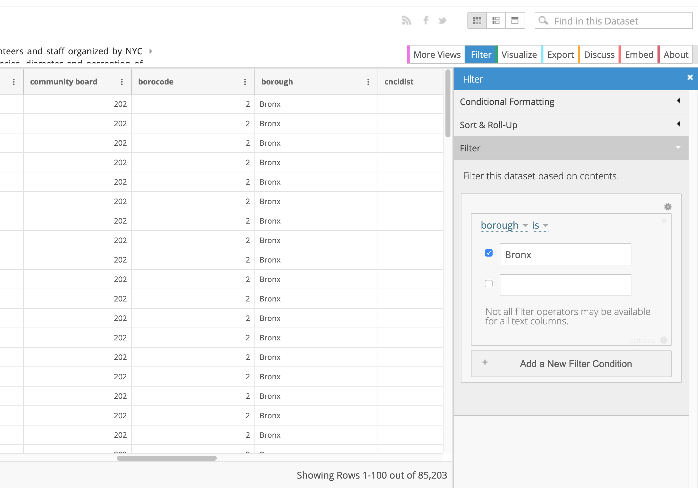

  

• Once the query runs, you should see that there are around 85,000 rows left. To download this subset of the data click Export and select CSV.

Adding a CSV File with Coordinates to QGIS

Before actually adding the CSV file to the map it is good practice to load and setup the other layers:

• Open a new QGIS map and add the Boroughs layer. Adding this layer first will make sure the map takes on the standard New York City projection (EPSG:2263 - NAD 83 / New York Long Island (ftUS)).

• Next, add the New York State Block Group layer.

• Finally, create a subset of the Block Group layer with only the block groups for the Bronx:

  • To do this, right-click the Block Group layer and open its attribute table.

  • Once there, click on the Select features using an expression button, the one with an ε on top of a yellow square.

  • In the next menu type the following query "COUNTYFP" = '005' and hit Select features. You should have 1154 features selected.

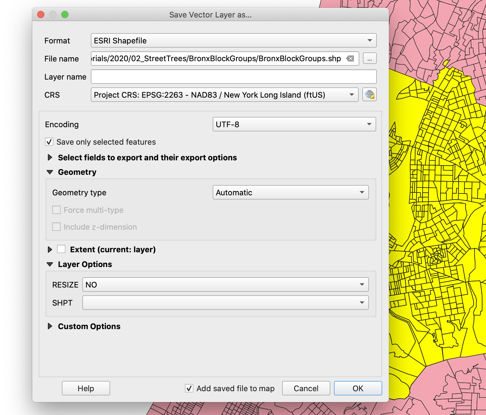
  • Close the attribute table and right-click on the Block Group layer. Select Export and then Save Selected Features As.... In the export menu make sure to choose EPSG:2263 - NAD 83 / New York Long Island (ftUS) as the export CRS.

  • Also, make sure you choose ESRI Shapefile as the format and you choose the right folder to export your file to.

  • Finally, make sure Save only selected features is checked.

  

• Once you have the layer for the Bronx block groups you can remove the New York State block groups.

• Now you can add the .csv file with the Bronx trees:

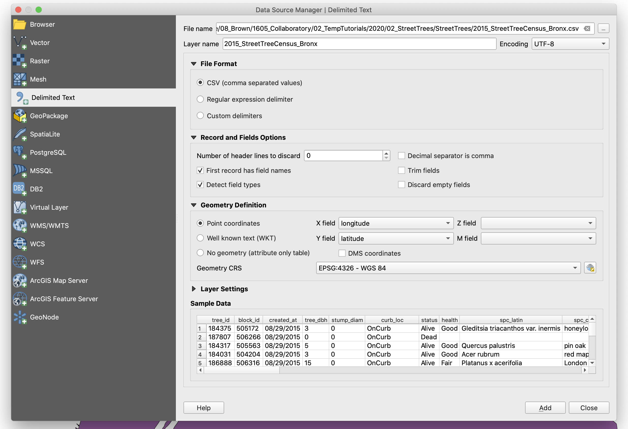
  • To add a .csv file click on the Add delimited text layer button (the one with the comma and +). You’ll see a window that is very similar to the one to import a vector layer.

  • Select the file and make sure the following presets are checked:

    • CSV (comma separated values)

    • Number of header lines to discard: 0

    • First record has field names

    • Detect field types

    • Point coordinates

    • X field: longitude

    • Y field: latitude

    • Geometry CRS: EPSG:4326 - WGS 84

    

  • Once you click Add and hit Close you should see your tree points on the map.

Counting Points in Polygons

• Before we run the algorithm for counting points in polygons it is always good practice to have your layers be in the same coordinate reference system. In our case, the polygon layer (Bronx block groups) is in EPSG:2263 and our tree layer is in EPSG:4326. They both look correct on the map because QGIS is transforming ‘on the fly` the tree layer to match the projection of the map. However, having layers in different coordinate reference systems can make operations take longer and be imprecise.

• To change the coordinate reference system of the tree layer, simply right-click on the layer and select Export, Save Features As.... In the export menu, select ESRI Shapefile and EPSG:2263 - NAD 83 / New York Long Island (ftUS) as the export CRS.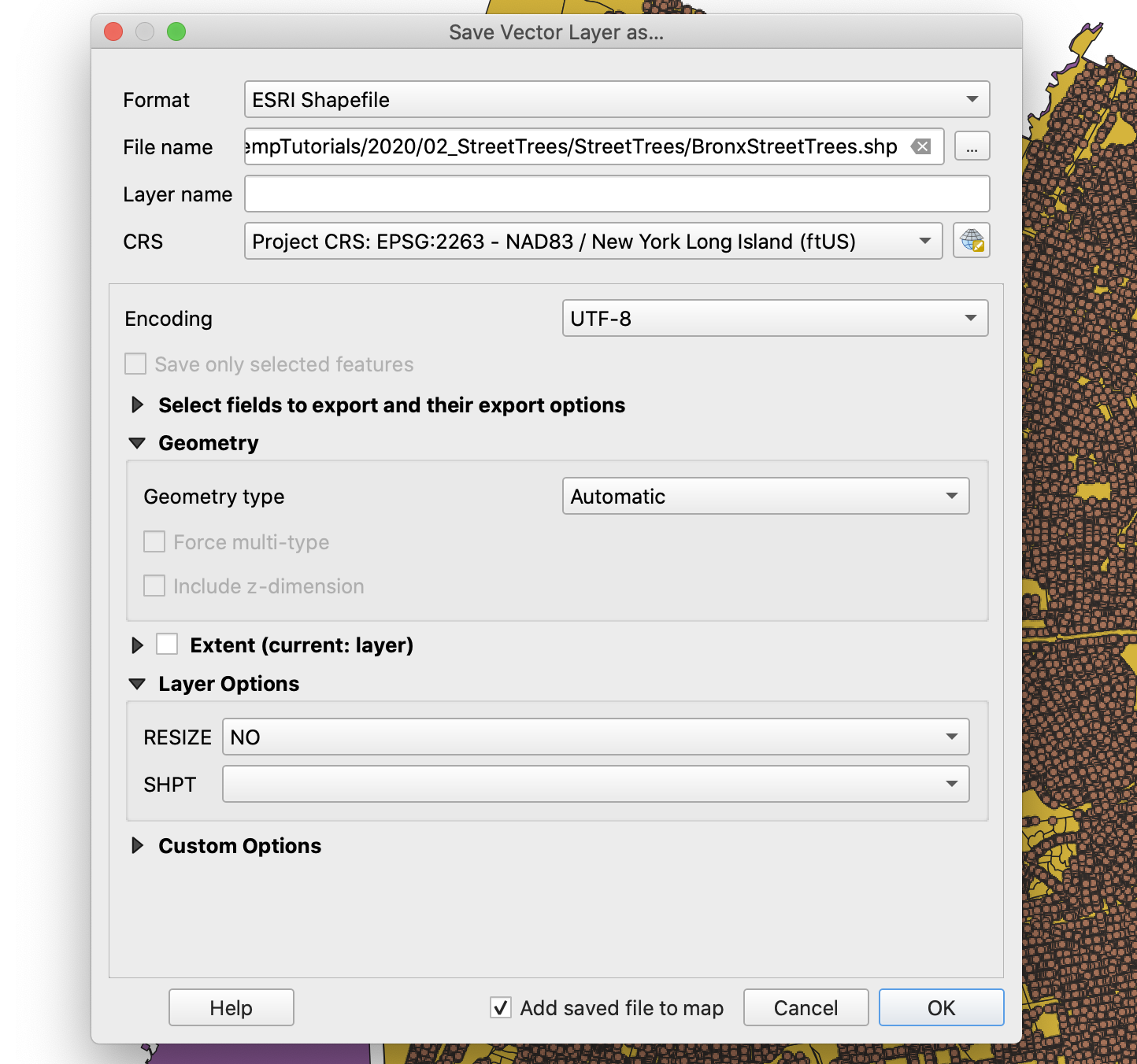

  

• Now that you have your new layer in you can remove the original tree data layer.

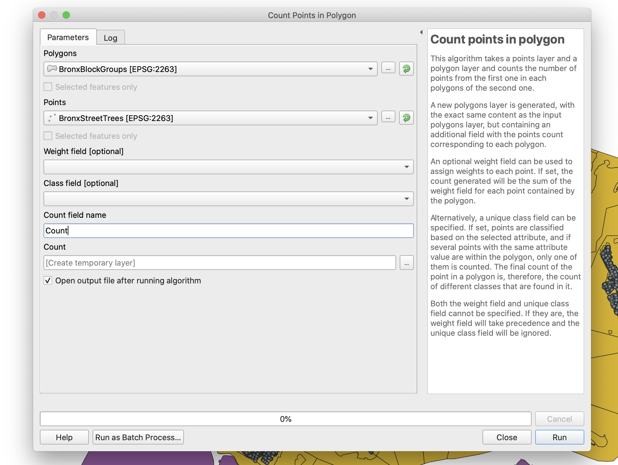
• Next, click on Vector, Analysis Tools, Count Points in Polygon:

• In the next menu choose:

  • Polygons: Bronx block groups layer

  • Points: Bronx street trees layer (make sure both the trees and the block groups layer have the same EPSG)

  • Count field name: Count

  

• Hit Run. The process might take a while (in preparing this tutorial it took around 3 minutes), but once it’s done you should have a new temporary layer of Bronx block groups with a new field for the number of trees in that block group.

• To make sure the operation was successful, open the attribute table of the new layer and move all the way to the right. You should see a column called Count with values for the number of trees.

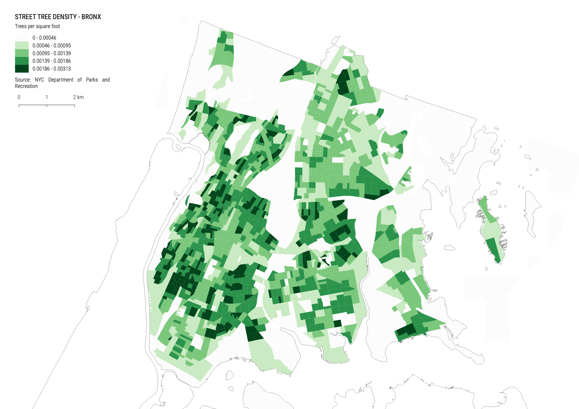
Calculating Tree Density

Now that we have the number of trees in each block group for the Bronx we could start symbolizing these values. However, notice that the sizes of the block groups vary greatly. It wouldn’t be fair to compare the number of trees in huge block groups with that of smaller block groups. It is always good practice to normalize your data. In this case we will do it by the size (square feet) of each block group.

• Before that, you should right click on your new Count layer and export it as its own shapefile. Right now, it is only a temporary layer, and if by any reason QGIS crashes or you close the program you will loose it.

• Once you have exported the layer you can remove all other layers except the boroughs. You’ll be left with your new Bronx block groups with tree count layer and the boroughs layer.

• To figure out the size of each block group we need to create the field and run the calculation:

  • Right-click on the layer and open the attribute table. Once there click on the Open field calculator button (the one with the abacus sign).

  • In the next menu, make sure the [x] Create a new field is checked.

  • Use SqFt as the output field name.

  • Choose Decimal number (real) as the output field type.

  • In the expression box type $area. This will automatically calculate the area of each feature. We know that the results will be in square feet because the projection we are using, EPSG:2263 - NAD 83 / New York Long Island (ftUS), uses feet as its unit.

  • Click OK to perform the operation. Once the calculation is done you will see a new field on the attribute table with the values for the area of each feature.

  • Finally, we need to calculate a new field for the tree density value (trees per square foot). Go through the same process to create a new field with this value. Make sure your output field type is Decimal number (real), your Precision is at least 6, and in the expression box type "Count" / "Sqft".

  • Once that calculation is done you should have your new TreeDen field. If everything is correct, click on the pencil icon at the top left of the attribute table to save your edits to the data. Now we are ready to symbolize.

Graduated Symbology

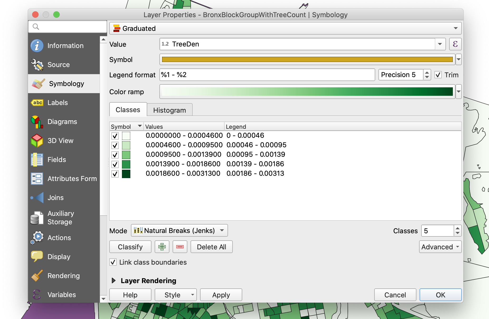
• To display our tree density values right-click on the block group layer and go to Properties.... There, choose the Symbology tab.

• In the first dropdown menu choose Graduated and in the Value menu choose the TreeDen column.

• Next hit the Classify button:

  • By default QGIS uses 5 buckets and an Equal Count (Quantile) method. There are in total 6 different methods of breaking up values into different buckets. Each one of them has its advantages and disadvantages and you should choose them very carefully as they might tell very different stories about your data. Depending on the ‘shape’ of your data and what you want to show, you should choose your classification method. Here’s a very brief explanation of the most common classification methods (taken from ArcGIS):

    • Equal Count (Quantile): In a quantile classification Quantile Class each class contains an equal number of features. A quantile classification is well suited to linearly distributed data. Quantile assigns the same number of data values to each class. There are no empty classes or classes with too few or too many values. Because features are grouped in equal numbers in each class using quantile classification, the resulting map can often be misleading. Similar features can be placed in adjacent classes, or features with widely different values can be put in the same class. You can minimize this distortion by increasing the number of classes.

    • Equal interval: Use equal interval Equal Interval to divide the range of attribute values into equal-sized subranges. This allows you to specify the number of intervals, and the class breaks based on the value range are automatically determined. For example, if you specify three classes for a field whose values range from 0 to 300, three classes with ranges of 0–100, 101–200, and 201–300 are created. Equal interval is best applied to familiar data ranges, such as percentages and temperature. This method emphasizes the amount of an attribute value relative to other values. For example, it shows that a shop is part of the group of shops that make up the top one-third of all sales.

    • Natural breaks (Jenks): With natural breaks classification (Jenks) Natural Breaks Jenks, classes are based on natural groupings inherent in the data. Class breaks are identified that best group similar values and that maximize the differences between classes. The features are divided into classes whose boundaries are set where there are relatively big differences in the data values. Natural breaks are data-specific classifications and not useful for comparing multiple maps built from different underlying information. This classification is based on the Jenks Natural Breaks algorithm.

    • Standard deviation: The standard deviation classification method Standard Deviation shows you how much a feature’s attribute value varies from the mean. The mean and standard deviation are calculated automatically. Class breaks are created with equal value ranges that are a proportion of the standard deviation—usually at intervals of one, one-half, one-third, or one-fourth standard deviations using mean values and the standard deviations from the mean.

  • To see the different results each classification method produces you should choose a classification method and then click the Histogram button, and then Load Values. There, you will see the shape of your data and how the classification method is breaking it into different buckets. You should also see the results on the map.

  • For this type of data the Natural breaks (Jenks) classification method is usually the best.

  • Finally, choose an appropriate color ramp.

  

Final Map Design

Once you have your data classify the only thing left to do is to add the other necessary layers (hydrography), style them, and put everything together in the Print Layout.

Your final map should look something like this: